
I am using example from my book “Finite Element Analysis using Open Source Software”. The example is of a 3D assembly of Guide and Weld. Let us look at how to generate a command file for a 3D assembly analysis of a simple Cantilevered beam and weld.
This beam is a Solid Rectangular with dimensions of 150 x 100 x 5 (Long x Width x Thickness). It has a 6mm fillet weld all around it.
Some important information regarding Assembly analysis is that the parts that need to be assembled should be in Master Slave pair.

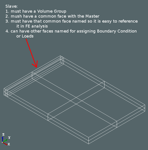
The faces that are common between Master and Slave should be on Slave

One face of the fillet weld is fixed and other face is used to connect to the Solid Rectangular Plate. A load of 2000N is applied on the other face of Plate.
Fixed face on the Weld is given a Mesh group name of “Fix”, the face on Guide on which Load is applied is given a Mesh group name of “Load” and the connecting face on Guide is given a name “f_Guide”
The meshes are named “v_weld” for Weld mesh and “v_guide” for Guide mesh and they are in MED format
So lets start generating command file for this analysis
Note: All screenshots are from a Windows 7 machine, using a different Operating system will not change the command file.
Step1:
Start Efficient (Click Here to see how to do that)
On the first tab, keep everything as default shown in screenshot below

Step2:
Click on Tab “Analysis Type” where we will select “Mechanical – 3D Assembly” in the left-top drop down box (highlighted yellow in screenshot below) and you will see that Information about Assembly will change colour from Red to White.
Step 2.1:
We need to make Code_Aster aware that there are two meshes that we want in this analysis. For this we add them to the command file with a Mesh Name and Number. In the screenshot below you can see that I have already added Mesh for Weld with a number 20. To add another Mesh, enter the name in Mesh Name, I have entered “v_guide” and Number (LU), I have added 21. Click on “Add Mesh Name and No.” and the mesh will be added to the command file.
Step 2.2:
Next we need to add how these two meshes are connected. For this we need to add Master – Slave pair. For a 3D Assembly analysis, a Master is a volume group which is “v_weld” for our case and a Slave is a Face group which is “f_guide” for our case. Enter these names in Master and Slave respectively and Click on “Add Master Slave Pair”.

Step3:
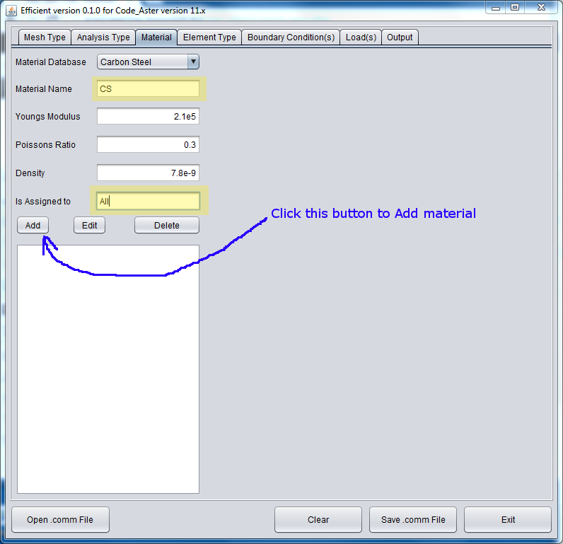
Click on Tab “Material” where we will add material to the analysis.
Enter “CS” for the Material Name
Keep default Youngs Modulus of 2.1e5 which is in MPa, Poisson’s Ratio of 0.3 and Density of 7.8e-9 (tonnes/mm^3)
Enter “All” for Is assigned to, to specify that entire Beam has this material.
Click on “Add” and the material will be added to the command file
Step4:
In 3D Assembly analysis we do not need to add Element Type, so leave this option blank.
Step5:
Click on Tab “Boundary Condition(s)” where we will add information about the Fixed Boundary Condition on mesh v_weld to the analysis.
Select “D.O.F (DDL) on Mesh Group” for Type of Boundary Cond. as we are adding a boundary condition on Group of Mesh
Enter “Fixed” for Boundary Condition Name. This is required as this name will be used in the command file from now on. This can be the same as the Mesh Group name defined in the mesh, but it does not need to be the same. Make sure the length of the Boundary Condition Name is less than or equal to 8 (Limitation of Fortran).
Enter “Fix” for Is assigned to, which is the name of the Mesh Group name defined in the mesh. This has to be exactly the same name (case sensitive) as given in the mesh.
Enter “0” (Zero) for all DX, DY and DZ and leave DRX, DRY and DRZ blank as we only need to add 3 degrees of freedom for a 3D element.
Click on “Add” and the boundary condition will be added to the command file.

Step6:
Click on Tab “Load(s)” where we will add information about the Loads to be applied to the analysis.
Enter “ForceZ” for Load Name, This is required as this name will be used in the command file from now on. This can be the same as the Mesh Group name defined in the mesh, but it does not need to be the same. Make sure the length of the Load Name is less than or equal to 8 (Limitation of Fortran).
Select “Force on Face” for Load Type as we will be applying a Force on a Face.
Enter “Load” for Is Assigned to, which is the name of the Mesh Group name defined in the mesh. This has to be exactly the same name (case sensitive) as given in the mesh.
As discussed in 3D analysis command file the Force to be applied is 2.
Enter “2” for FZ.
Click on “Add” and the load will be added to the command file.

Step7:
Click on Tab “Output” where we will add information about the types of results that we want in the analysis.
Efficient is intelligent to know that the type of Analysis is “3D Assembly” which has same results to a “3D” analysis and so it showed only those output Options that are related to 3D continuum analysis.
If you don’t ADD anything in this Tab, only Deflection will be saved in MED file
As we want all options that are available for this Analysis we will click “Add ALL”

Step8:
Now the only thing left is the Click “Save .comm File”, Efficient will ask for a location where you want to save this file, select a folder where you want the file to be saved and give it a name, Here I have given it a name “3D-Assembly.comm”. (Remember to add .comm at the end of the File name as by default this is not written by Efficient.

Click on “Save” and the file will be saved. Once Efficient has saved the file, it will show message as follows

Hurray, you have a working command file within few seconds.
Your comm file should look like below
###############################
#File created by Efficient Software version 0.1.0
#Version of Code_Aster is 11.x
#Author of Efficient is Dhramit Thakore
#https://engineering.moonish.biz
###############################
#U4.11.01
#@Eff@#StartCont#DEBUT
DEBUT();
#U4.21.01
#@Eff@#MeshType#MED
#@Eff@#MeshNameAndLU#v_weld;20
v_weld=LIRE_MAILLAGE(UNITE=20, FORMAT='MED',);
#@Eff@#MeshNameAndLU#v_guide;21
v_guide=LIRE_MAILLAGE(UNITE=21, FORMAT='MED',);
mesh=ASSE_MAILLAGE(MAILLAGE_1=v_weld, MAILLAGE_2=v_guide, OPERATION='SUPERPOSE',);
#U4.41.01
#@Eff@#AnalysisType#Mechanical - 3D Assembly
model=AFFE_MODELE(MAILLAGE=mesh, AFFE=_F(TOUT='OUI', PHENOMENE='MECANIQUE', MODELISATION='3D',),);
#U4.43.01
#@Eff@#MaterialList#CS;2.1e5;0.3;7.8e-9;All
CS=DEFI_MATERIAU(ELAS=_F(E=2.1e5, NU=0.3, RHO=7.8e-9,),);
#U4.43.03
material=AFFE_MATERIAU(MAILLAGE=mesh, AFFE=(_F(TOUT='OUI', MATER=CS,),),);
#U4.44.01
#@Eff@#BCList#D.O.F (DDL) on Mesh Group;Fixed;Fix;0;0;0;NA;NA;NA;NA;NA
Fixed=AFFE_CHAR_MECA(MODELE=model, DDL_IMPO=_F(GROUP_MA='Fix',DX=0,DY=0,DZ=0,),);
#@Eff@#MasterSlaveList#v_weld;f_guide
combine=AFFE_CHAR_MECA(MODEL=model, LIAISON_MAIL=(
 _F(GROUP_MA_MAIT='v_weld', GROUP_MA_ESCL='f_guide', TYPE_RACCORD='MASSIF',),
),);
#U4.44.01
#@Eff@#LoadList#ForceZ;Force on Face;Load;NA;NA;2;NA;NA;NA
ForceZ=AFFE_CHAR_MECA(MODELE=model, FORCE_FACE=(_F(GROUP_MA='Load', FZ = 2,),),);
result=MECA_STATIQUE(MODELE=model, CHAM_MATER=material, EXCIT=(_F(CHARGE=Fixed,),_F(CHARGE=combine,),_F(CHARGE=ForceZ,),),);
#U4.81.04
result=CALC_CHAMP(reuse=result, RESULTAT=result, CONTRAINTE=('SIGM_ELNO','SIGM_NOEU',), CRITERES=('SIEQ_ELNO','SIEQ_NOEU',), FORCE=('REAC_NODA',),);
#U4.91.01
#@Eff@#OutputMEDList#SIGM_ELNO
#@Eff@#OutputMEDList#SIGM_NOEU
#@Eff@#OutputMEDList#SIEQ_ELNO
#@Eff@#OutputMEDList#SIEQ_NOEU
#@Eff@#OutputMEDList#REAC_NODA
IMPR_RESU(FORMAT='MED', UNITE=80, RESTREINT=_F(GROUP_MA='v_weld',), RESU=_F(MAILLAGE=mesh, RESULTAT=result, NOM_CHAM=('DEPL', 'SIGM_ELNO', 'SIGM_NOEU', 'SIEQ_ELNO', 'SIEQ_NOEU', 'REAC_NODA',),),);
IMPR_RESU(FORMAT='MED', UNITE=81, RESTREINT=_F(GROUP_MA='v_guide',), RESU=_F(MAILLAGE=mesh, RESULTAT=result, NOM_CHAM=('DEPL', 'SIGM_ELNO', 'SIGM_NOEU', 'SIEQ_ELNO', 'SIEQ_NOEU', 'REAC_NODA',),),);
#U4.11.02
FIN();
Review this file carefully as quiet a few things have changed in it. To get more insights on what is the meaning of each line in the command file, have a look at my book “Finite Element Analysis using Open Source Software”.